Combining Stations (Plan B)

In his post on combining  station monthly temperature series, Tamino proposes a method for calculating an “offset” for each station.  This offset is intended to place the series for the stations all on at the same level.  The reason that makes such an accommodation necessary is the fact that there are often missing values in a given record – sometimes for complete years at a stretch.   Simple averages  in such a situation can provide a distorted view of what the overall picture looks like.

In his proposed “optimal” method, Tamino suggests  a procedure based on least square methods to calculate a set of coefficients for shifting a station record up or down before calculating a combined series for the set of stations.  The starting point is a sum of squares (which for calculational and discussion purposes I have rewritten in a slightly different form):

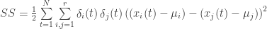
Here,

i (and j)  = 1, 2, …, r, = the station identifiers for a set of r stations

t = 1, 2, …, N, = the time (i.e. year and month) of the observation

x_i(t) = the observed temperature at station i at time t

µ_i = the offset  value which is subtracted from station i

δ_i(t) = indicator of whether x_i(t) is missing (0) or available (1)

In essence, the Sum of Squares measures the squared differences between the “adjusted” temperatures of every pair of available stations at each time with each pair weighted equally.  The estimated offsets minimize this sum.  The mathematically adept person will recognize that the solution for the individual µ’s is not unique, however the differences between them are.  Tamino chooses to set µ₁ = 0 to choose a specific solution.

All available adjusted values are averaged at each time t to form a combined temperature series.  This can then be transformed into anomaly series or otherwise manipulated.

On the surface this seems like a straightforward thing to do, but, for a statistician, it leaves a lot to be desired.  The principle of minimizing the given SS is not bad.  Bringing the station series as close as possible to each other is a good idea.  What is missing is a context – call it a mathematical model – within which one can identify and interpret the results obtained.  What exactly do the results represent?  What does the random variability structure of the data look like?  Is the simple average of the adjusted values the best thing to do? How can one calculate error bars for the estimates (particularly if the randomness structure of the data is complicated)?  Can this structure be re-stated in a different way which allows for the answer to the previous questions?

The Model

Starting with the Sum of Squares above and using some genuine ( 🙂 ) mathematical tricks, I did some “reverse engineering”.  I won’t give the mathematical derivation here, although it is not all that difficult to do (although there would be a lot of equations to write out).  Instead, I will give the end result:

Using similar notation to that above, the temperatures can be expressed as

τ(t)  = the actual combined temperature series

µ_i = the offset  amount by which the station differs from  the combined temperatures

ε_i(t) = the “error” (i.e. random term) in the measurement

This is basically what might be termed a two factor Analysis of Variance.  However, the reverse engineering indicates that in order to stay with achieving offsets which are the same as those which minimize Tamino’s SS,  we need to weight the station temperature x_i(t) with a weight proportional to

ω_i(t) = the number of available stations at time t

Thus the appropriate “weighted” sum of squares to be minimized is

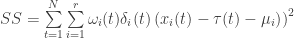
Now, this SS is minimized by exactly the same values which are calculated by Tamino’s procedure (proof, at this point in time, is left to the reader 😉 ).  First, one can minimize the first SS for the estimated µ’s and then average the adjusted values to estimate the τ(t)’s.    Alternatively, one can just run the appropriate procedure in R (or another program) to directly get not only the estimates of the parameters, but to get confidence error bars or to do statistical tests as well.  The advantage of rewriting the problem in this fashion has been the ability to answer the questions that were raised above.

So Tamino got it right? Well, not exactly…

Plan B: A “More Optimal” Model

The model above (along with Tamino) assumes that the difference between a pair stations is a constant throughout the year.  For geographical reasons, this may not be true much of the time even for stations that are relatively close.  Examples of this would be a station in a coastal area compared to one farther inland.  The coastal station will likely vary less during the year: cooler summers and warmer winters than the one farther inland.  There can also be such differences observed due to a difference in altitude.   If Tamino had looked at the residuals (temperatures minus sum of combined series and offsets) of the example series in his post , he would have noticed a pronounced annual periodicity.  One might argue that this would disappear (it won’t since only the τ(t)’s would be used) if the resulting combined series is somehow anomalized, but the difficulty goes much deeper.

The reason for the necessity of this procedure is the presence of missing values.   When a single offset is used, not only will a noiseless set of periodic series (with varying monthly differences) be unable to reconstruct the mean series as values are removed, but the size of the error in the estimated value  will also depend on which months are missing.

Fortunately, the solution is simple.  Instead of a single offset for a station, we can calculate one for each month:

m(t) = the month at time t

Our derivation above is not wasted since we can simply subdivide the time series by month and use the earlier calculation methodology to carry out the estimation procedure for each monthly series.  The results are then concatenated back together to form the final combined series.

In my opinion, this is a pretty reasonable approach to use since there are other bonuses here as well.  A graphical analysis of the residuals for each station can give insight about possible changes at a station whether such changes are instantaneous steps or prolonged slow increases (such as UHI) or decreases.  The model can also be altered to test whether known alterations at a station have produced step changes.

I have written some scripts both from direct programming of the initial Tamino approach as well as using R’s lm procedure. The following script uses the anova model described directly above. The µ’s are centered so that the mean of all the station offsets for each month is equal to zero. If there are no missing stations at a given time, this has the effect of defining τ(t) to be the mean of all the individual temperature series.

It is possible that there may be an occasional bug in the script so please inform me if you find something amiss. If necessary, I can also tart up the script which I wrote initially for directly calculating the various estimates (both in the single offset and the multiple offset cases) to make it “turnkey” in its operation and post it. I also did not run examples of the use of the script because the post would have become too long. I will try to to run of some of these in the near future if there appears to be sufficient interest.

[Update:  Further analysis has shown that this method is NOT optimal.   please see Combining Stations – Plan C]

###  anov.combine = Function to do monthly anova
## Input:
#  ttemp = multivariate time series

## Output:
#  temps = combined temperature series
#  offsets = monthly offsets for each station
#  residual = multivariate resuidual time series
#  predicted = predicted temperatures
#  Note:  ttemp = predicted + residual

anov.combine = function(ttemp,anom=F) {
#function to restructure data for anova
  conv.anov = function(ind.var) {
    dims.ind = dim(ind.var)
    response = c(ind.var)
    rowvar = as.factor(c(row(ind.var)))
    colvar = as.factor(c(col(ind.var)))
    months = as.factor(rep(1:12,len=nrow(ind.var)))
    weights = ncol(ind.var)-rowSums(is.na(ind.var))
    data.frame(response=response, rowvar=rowvar, colvar=colvar, months=months, weights=weights)}
  datanov = conv.anov(ttemp)
#calculate anovas by month
   anovout = by(datanov, datanov$months, function(x) lm(response~0+rowvar+colvar,data=x,weights=weights))
   offs = matrix(NA,12,ncol(ttemp))
   temp.ts = rep(NA,nrow(ttemp))
 for (i in 1:12) { testco = coef(anovout[[i]])
  whch = grep("rowvar",names(testco))
  temp.ts[as.numeric(substr(names(testco)[whch],7,11))] = testco[whch]-anom*testco[whch[1]]
  offs[i,] = c(0,testco[grep("colvar",names(testco))])}
#center offsets and adjust time series
  nr = length(temp.ts)
  adj = rowMeans(offs)
  offs = offs-adj
  temp.ts = temp.ts + rep(adj, length=nr)
#calculate predicted and residuals for data
   nc = ncol(offs)
   matoff = matrix(NA,nr,nc)
  for (i in 1:nc) matoff[,i] = rep(offs[,i],length=nr)
   preds = c(temp.ts) + matoff
  temps = ts(temp.ts)
  tsp(temps) = tsp(ttemp)
 colnames(offs) = colnames(ttemp)
 rownames(offs) = month.abb
list(temps = temps,offsets = offs, residual = ttemp - preds, predicted=preds) }

### anomaly.calc = Function to convert temperature time series to anomalies
## Input:
#  tsdat = univariate temperature time series

## Output:
#  anomaly temperature series

anomaly.calc=function(tsdat,styr=1951,enyr=1980){
  tsmeans = rowMeans(matrix(window(tsdat,start=c(styr,1),end=c(enyr,12)),nrow=12))
  tsdat-rep(tsmeans,length=length(tsdat))}